武汉夜生活网论坛|武汉桑拿论坛|武汉027狼盟

Black holes are extremely camera shy. Supermassive black holes, ensconced in the centers of galaxies, make themselves visible by spewing bright jets of charged particles or by flinging away or ripping up nearby stars. Up close, these behemoths are surrounded by glowing accretion disks of infalling material. But because a black hole’s extreme gravity prevents light from escaping, the dark hearts of these cosmic heavy hitters remain entirely invisible.

Luckily, there’s a way to “see” a black hole without peering into the abyss itself. Telescopes can look instead for the silhouette of a black hole’s event horizon — the perimeter inside which nothing can be seen or escape — against its accretion disk. That’s what the Event Horizon Telescope, or EHT, did in April 2017, collecting data that has now yielded the first image of a supermassive black hole, the one inside the galaxy M87.

“There is nothing better than having an image,” says Harvard University astrophysicist Avi Loeb. Though scientists have collected plenty of indirect evidence for black holes over the last half century, “seeing is believing.”

Creating that first-ever portrait of a black hole was tricky, though. Black holes take up a minuscule sliver of sky and, from Earth, appear very faint. The project of imaging M87’s black hole required observatories across the globe working in tandem as one virtual Earth-sized radio dish with sharper vision than any single observatory could achieve on its own.
Putting the ‘solution’ in resolution
Weighing in around 6.5 billion times the mass of our sun, the supermassive black hole inside M87 is no small fry. But viewed from 55 million light-years away on Earth, the black hole is only about 42 microarcseconds across on the sky. That’s smaller than an orange on the moon would appear to someone on Earth. Still, besides the black hole at the center of our own galaxy, Sagittarius A* or Sgr A* — the EHT’s other imaging target — M87’s black hole is the largest black hole silhouette on the sky.
Only a telescope with unprecedented resolution could pick out something so tiny. (For comparison, the Hubble Space Telescope can distinguish objects only about as small as 50,000 microarcseconds.) A telescope’s resolution depends on its diameter: The bigger the dish, the clearer the view — and getting a crisp image of a supermassive black hole would require a planet-sized radio dish.
Even for radio astronomers, who are no strangers to building big dishes (SN Online: 9/29/17), “this seems a little too ambitious,” says Loeb, who was not involved in the black hole imaging project. “The trick is that you don’t cover the entire Earth with an observatory.”
Instead, a technique called very long baseline interferometry combines radio waves seen by many telescopes at once, so that the telescopes effectively work together like one giant dish. The diameter of that virtual dish is equal to the length of the longest distance, or baseline, between two telescopes in the network. For the EHT in 2017, that was the distance from the South Pole to Spain.

Telescopes, assemble!
The EHT was not always the hotshot array that it is today, though. In 2009, a network of just four observatories — in Arizona, California and Hawaii — got the first good look at the base of one of the plasma jets spewing from the center of M87’s black hole (SN: 11/3/12, p. 10). But the small telescope cohort didn’t yet have the magnifying power to reveal the black hole itself.

Over time, the EHT recruited new radio observatories. By 2017, there were eight observing stations in North America, Hawaii, Europe, South America and the South Pole. Among the newcomers was the Atacama Large Millimeter/submillimeter Array, or ALMA, located on a high plateau in northern Chile. With a combined dish area larger than an American football field, ALMA collects far more radio waves than other observatories.

“ALMA changed everything,” says Vincent Fish, an astronomer at MIT’s Haystack Observatory in Westford, Mass. “Anything that you were just barely struggling to detect before, you get really solid detections now.”
More than the sum of their parts
EHT observing campaigns are best run within about 10 days in late March or early April, when the weather at every observatory promises to be the most cooperative. Researchers’ biggest enemy is water in the atmosphere, like rain or snow, which can muddle with the millimeter-wavelength radio waves that the EHT’s telescopes are tuned to.

But planning for weather on several continents can be a logistical headache.

“Every morning, there’s a frenetic set of phone calls and analyses of weather data and telescope readiness, and then we make a go/no-go decision for the night’s observing,” says astronomer Geoffrey Bower of the Academia Sinica Institute of Astronomy and Astrophysics in Hilo, Hawaii. Early in the campaign, researches are picky about conditions. But toward the tail end of the run, they’ll take what they can get.

When the skies are clear enough to observe, researchers steer the telescopes at each EHT observatory toward the vicinity of a supermassive black hole and begin collecting radio waves. Since M87’s black hole and Sgr A* appear on the sky one at a time — each one about to rise just as the other sets — the EHT can switch back and forth between observing its two targets over the course of a single multi-day campaign. All eight observatories can track Sgr A*, but M87 is in the northern sky and beyond the South Pole station’s sight.

On their own, the data from each observing station look like nonsense. But taken together using the very long baseline interferometry technique, these data can reveal a black hole’s appearance.

Here’s how it works. Picture a pair of radio dishes aimed at a single target, in this case the ring-shaped silhouette of a black hole. The radio waves emanating from each bit of that ring must travel slightly different paths to reach each telescope. These radio waves can interfere with each other, sometimes reinforcing one another and sometimes canceling each other out. The interference pattern seen by each telescope depends on how the radio waves from different parts of the ring are interacting when they reach that telescope’s location.
For simple targets, such as individual stars, the radio wave patterns picked up by a single pair of telescopes provide enough information for researchers to work backward and figure out what distribution of light must have produced those data. But for a source with complex structure, like a black hole, there are too many possible solutions for what the image could be. Researchers need more data to work out how a black hole’s radio waves are interacting with each other, offering more clues about what the black hole looks like.

The ideal array has as many baselines of different lengths and orientations as possible. Telescope pairs that are farther apart can see finer details, because there’s a bigger difference between the pathways that radio waves take from the black hole to each telescope. The EHT includes telescope pairs with both north-south and east-west orientations, which change relative to the black hole as Earth rotates.

Pulling it all together
In order to braid together the observations from each observatory, researchers need to record times for their data with exquisite precision. For that, they use hydrogen maser atomic clocks, which lose about one second every 100 million years.

There are a lot of data to time stamp. “In our last experiment, we recorded data at a rate of 64 gigabits per second, which is about 1,000 times [faster than] your home internet connection,” Bower says.

These data are then transferred to MIT Haystack Observatory and the Max Planck Institute for Radio Astronomy in Bonn, Germany, for processing in a special kind of supercomputer called a correlator. But each telescope station amasses hundreds of terabytes of information during a single observing campaign — far too much to send over the internet. So the researchers use the next best option: snail mail. So far, there have been no major shipping mishaps, but Bower admits that mailing the disks is always a little nerve-wracking.

Though most of the EHT data reached Haystack and Max Planck within weeks of the 2017 observing campaign, there were no flights from South Pole until November. “We didn’t get the data back from the South Pole until mid-December,” says Fish, the MIT Haystack astronomer.

Filling in the blanks
Combining the EHT data still isn’t enough to render a vivid picture of a supermassive black hole. If M87’s black hole were a song, then imaging it using only the combined EHT data would be like listening to the piece played on a piano with a bunch of broken keys. The more working keys — or telescope baseline pairs — the easier it is to get the gist of the melody. “Even if you have some broken keys, if you’re playing all the rest of them correctly, you can figure out the tune, and that’s partly because we know what music sounds like,” Fish says. “The reason we can reconstruct images, even though we don’t have 100 percent of the information, is because we know what images look like” in general.
There are mathematical rules about how much randomness any given picture can contain, how bright it should be and how likely it is that neighboring pixels will look similar. Those basic guidelines can inform how software decides which potential images, or data interpretations, make the most sense.

Before the 2017 observing campaign, the EHT researchers held a series of imaging challenges to make sure their computer algorithms weren’t biased toward creating images to match expectations of what black holes should look like. One person would use a secret image to generate faux data of what telescopes would see if they were peering at that source. Then other researchers would try to reconstruct the original image.

“Sometimes the true image was not actually a black hole image,” Fish says, “so if your algorithm was trying to find a black hole shadow … you wouldn’t do well.” The practice runs helped the researchers refine the data processing techniques used to render the M87 image.

Black holes and beyond
So, the black hole inside M87 finally got its closeup. Now what?

The EHT’s black hole observations are expected to help answer questions like how some supermassive black holes, including M87’s, launch such bright plasma jets (SN Online: 3/29/19). Understanding how gas falls into and feeds black holes could also help solve the mystery of how some black holes grew so quickly in the early universe, Loeb says (SN Online: 3/16/18).

The EHT could also be used, Loeb suggests, to find pairs of supermassive black holes orbiting one another — similar to the two stellar mass black holes whose collision created gravitational waves detected in 2015 by the Advanced Laser Interferometer Gravitational-Wave Observatory, or Advanced LIGO (SN: 3/5/16, p. 6). Getting a census of these binaries may help researchers identify targets for the Laser Interferometer Space Antenna, or LISA, which will search from space for gravitational waves kicked up by the movement of objects like black holes (SN Online: 6/20/17).
The EHT doesn’t have many viable targets other than supermassive black holes, says astrophysicist Daniel Marrone, at the University of Arizona in Tucson. There are few other things in the universe that appear as tiny but luminous as the space surrounding a supermassive black hole. “You have to be able to get enough light out of the really tiny patches of sky that we can detect,” Marrone says. “In principle, we could be reading alien license plates or something,” but they’d need to be super bright.

Too bad for alien seekers. Still, even if the EHT is a one-trick pony, spying supermassive black holes is a pretty neat trick.

A new member of the human genus has been found in a cave in the Philippines, researchers report.

Fossils with distinctive features indicate that the hominid species inhabited the island now known as Luzon at least 50,000 years ago, according to a study in the April 11 Nature. That species, which the scientists have dubbed Homo luzonensis, lived at the same time that controversial half-sized hominids named Homo floresiensis and nicknamed hobbits were roaming an Indonesian island to the south called Flores (SN: 7/9/16, p. 6).
In shape and size, some of the fossils match those of corresponding bones from other Homo species. “But if you take the whole combination of features for H. luzonensis, no other Homo species is similar,” says study coauthor and paleoanthropologist Florent Détroit of the French National Museum of Natural History in Paris.

If the find holds up to further scientific scrutiny, it would add to recent fossil and DNA evidence indicating that several Homo lineages already occupied East Asia and Southeast Asian islands by the time Homo sapiens reached what’s now southern China between 80,000 and 120,000 years ago (SN: 11/14/15, p. 15). The result: an increasingly complicated picture of hominid evolution in Asia.

Excavations in 2007, 2011 and 2015 at Luzon’s Callao Cave yielded a dozen H. luzonensis fossils at first — seven isolated teeth (five from the same individual), two finger bones, two toe bones and an upper leg bone missing its ends, the scientists say. Analysis of the radioactive decay of uranium in one tooth suggested a minimum age of 50,000 years. Based on those fossils, a hominid foot bone found in 2007 in the same cave sediment was also identified as H. luzonensis. It dates to at least 67,000 years ago.
had molars that were especially small, even smaller than those of hobbits, with some features similar to modern humans’ molars. The hominid also had relatively large premolars that, surprisingly, had two or three roots rather than one. Hominids dating to several hundred thousand years ago or more, such as Homo erectus , typically had premolars with multiple roots. H. luzonensis finger and toe bones are curved, suggesting a tree-climbing ability comparable to hominids from 2 million years ago or more.
It’s unclear whether H. luzonensis was as small as hobbits, Détroit says. The best-preserved hobbit skeleton comes from a female who stood about a meter tall. Based on the length of the Callao Cave foot bone, Détroit’s team suspects that H. luzonensis was taller than that, although still smaller than most human adults today.

As with hobbits, H. luzonensis’ evolutionary origins are unknown. Scientists think that hobbits may have descended from seagoing H. erectus groups, and perhaps H. luzonensis did too, writes paleoanthropologist Matthew Tocheri of Lakehead University in Thunder Bay, Canada, in a commentary published with the new report. Evidence suggests that hominids reached Luzon by around 700,000 years ago (SN Online: 5/2/18). So H. erectus may have also crossed the sea from other Indonesian islands or mainland Asia to Luzon and then evolved into H. luzonensis with its smaller body and unusual skeletal traits, Détroit speculates, a process known as island dwarfing.

But some scientists not involved in the research say it’s too soon to declare the Luzon fossils a brand-new Homo species. Détroit’s group, so far, has been unable to extract ancient DNA from the fossils. So “all [evolutionary] possibilities must remain open,” says archaeologist Katerina Douka of the Max Planck Institute for the Science of Human History in Jena, Germany.

The mosaic of fossil features that the team interprets as distinctive, for instance, may have been a product of interbreeding between two or more earlier Homo species, creating hybrids, but not a new species.

Or perhaps a small population of, say, H. erectus that survived on an isolated island like Luzon for possibly hundreds of thousands of years simply acquired some skeletal features that its mainland peers lacked, rather than evolving into an entirely new species, says paleoanthropologist María Martinón-Torres.

Those questions make the new fossils “an exciting and puzzling discovery,” says Martinón-Torres, director of the National Research Centre on Human Evolution in Burgos, Spain.

If the unusual teeth and climbing-ready hand and foot bones found at Callao Cave occurred as a package among Luzon’s ancient Homo crowd, “then that combination is unique and unknown so far” among hominids, Martinón-Torres says. Only a more complete set of fossils, ideally complemented by ancient DNA, she adds, can illuminate whether such traits marked a new Homo member.

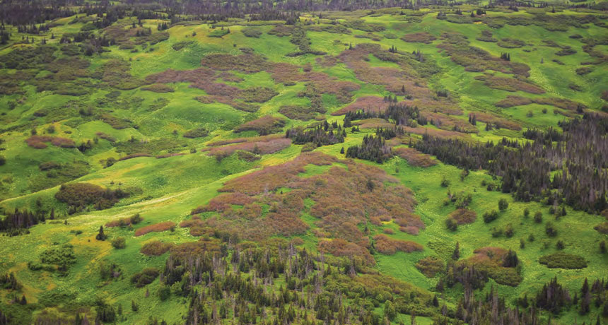
The Chugach people of southern Alaska’s Kenai Peninsula have picked berries for generations. Tart blueberries and sweet, raspberry-like salmonberries — an Alaska favorite — are baked into pies and boiled into jams. But in the summer of 2009, the bushes stayed brown and the berries never came.

For three more years, harvests failed. “It hit the communities very hard,” says Nathan Lojewski, the forestry manager for Chugachmiut, a nonprofit tribal consortium for seven villages in the Chugach region.
The berry bushes had been ravaged by caterpillars of geometrid moths — the Bruce spanworm (Operophtera bruceata) and the autumnal moth (Epirrita autumnata). The insects had laid their eggs in the fall, and as soon as the leaf buds began growing in the spring, the eggs hatched and the inchworms nibbled the stalks bare.

Chugach elders had no traditional knowledge of an outbreak on this scale in the region, even though the insects were known in Alaska. “These berries were incredibly important. There would have been a story, something in the oral history,” Lojewski says. “As far as the tribe was concerned, this had not happened before.”

At the peak of the multiyear outbreak, the caterpillars climbed from the berry bushes into trees. The pests munched through foliage from Port Graham, at the tip of the Kenai Peninsula, to Wasilla, north of Anchorage, about 300 kilometers away. In summer, thick brown-gray layers of denuded willows, alders and birches lined the mountainsides above stretches of Sitka spruce.
Two summers ago, almost a decade after the first infestation, the moths returned. “We got a few berries, but not as many as we used to,” says Chugach elder Ephim Moonin Sr., whose house in the village of Nanwalek is flanked by tall salmonberry bushes. “Last year, again, there were hardly any berries.”
For more than 35 years, satellites circling the Arctic have detected a “greening” trend in Earth’s northernmost landscapes. Scientists have attributed this verdant flush to more vigorous plant growth and a longer growing season, propelled by higher temperatures that come with climate change. But recently, satellites have been picking up a decline in tundra greenness in some parts of the Arctic. Those areas appear to be “browning.”
Like the salmonberry harvesters on the Kenai Peninsula, ecologists working on the ground have witnessed browning up close at field sites across the circumpolar Arctic, from Alaska to Greenland to northern Norway and Sweden. Yet the bushes bereft of berries and the tinder-dry heaths (low-growing shrubland) haven’t always been picked up by the satellites. The low-resolution sensors may have averaged out the mix of dead and living vegetation and failed to detect the browning.

Scientists are left to wonder what is and isn’t being detected, and they’re concerned about the potential impact of not knowing the extent of the browning. If it becomes widespread, Arctic browning could have far-reaching consequences for people and wildlife, affecting habitat and atmospheric carbon uptake and boosting wildfire risk.

Growing greenbelt
The Arctic is warming two to three times as fast as the rest of the planet, with most of the temperature increase occurring in the winter. Alaska, for example, has warmed 2 degrees Celsius since 1949, and winters in some parts of the state, including southcentral Alaska and the Arctic interior, are on average 5 degrees C warmer.

An early effect of the warmer climate was a greener Arctic. More than 20 years ago, researchers used data from the National Oceanic and Atmospheric Administration’s weather satellites to assess a decade of northern plant growth after a century of warming. The team compared different wavelengths of light — red and near-infrared — reflecting off vegetation to calculate the NDVI, the normalized difference vegetation index. Higher NDVI values indicate a greener, more productive landscape. In a single decade — from 1981, when the first satellite was launched, to 1991 — the northern high latitudes had become about 8 percent greener, the researchers reported in 1997 in Nature.

The Arctic ecosystem, once constrained by cool conditions, was stretching beyond its limits. In 1999 and 2000, researchers cataloged the extent and types of vegetation change in parts of northern Alaska using archival photographs taken during oil exploration flyovers between 1948 and 1950. In new images of the same locations, such as the Kugururok River in the Noatak National Preserve, low-lying tundra plants that once grew along the riverside terraces had been replaced by stands of white spruce and green alder shrubs. At some of the study’s 66 locations, shrub-dominated vegetation had doubled its coverage from 10 to 20 percent. Not all areas showed a rise in shrub abundance, but none showed any decrease.

In 2003, Howard Epstein, a terrestrial ecologist at the University of Virginia in Charlottesville, and colleagues looked to the satellite record, which now held another decade of data. Focusing on Alaska’s North Slope, which lies just beyond the crown of the Brooks Range and extends to the Beaufort Sea, the researchers found that the highest NDVI values, or “peak greenness,” during the growing season had increased nearly 17 percent between 1981 and 2001, in line with the warming trend.
Earth-observing satellites have been monitoring the Arctic tundra for almost four decades. In that time, the North Slope, the Canadian low Arctic tundra and eastern Siberia have become especially green, with thicker and taller tundra vegetation and shrubs expanding northward. “If you look at the North Slope of Alaska, if you look at the overall trend, it’s greening like nobody’s business,” says Uma Bhatt, an atmospheric scientist at the University of Alaska Fairbanks.

Yet parts of the Arctic, including the Yukon-Kuskokwim Delta of western Alaska, the Canadian Arctic Archipelago (the islands north of the mainland that give Canada its pointed tip) and the northwestern Siberian tundra, show extensive browning over the length of the satellite record, from the early 1980s to 2016. “It could just be a reduction in green vegetation. It doesn’t necessarily mean the widespread death of plants,” Epstein says. Scientists don’t yet know why plant growth there has slowed or reversed — or whether the satellite signal is in some way misleading.

“All the models indicated for a long time that we would expect greening with warmer temperatures and higher productivity in the tundra, so long as it wasn’t limited in some other way, like [by lower] moisture,” says Scott Goetz, an ecologist and remote-sensing specialist at Northern Arizona University in Flagstaff. He is also the science team lead for ABoVE, NASA’s Arctic-Boreal Vulnerability Experiment, which is tracking ecosystem changes in Alaska and western Canada. “Many of us were quite surprised … that the Arctic was suddenly browning. It’s something we need to resolve.”

Freeze-dried tundra
While global warming has propelled widespread trends in tundra greening, extreme winter weather can spur local browning events. In recent years, in some parts of the Arctic, extraordinary warm winter weather, sometimes paired with rainfall, has put tundra vegetation under enormous stress and caused plants to lose freeze resistance, dry up or die — and turn brown.

Gareth Phoenix, a terrestrial ecologist at the University of Sheffield in England, recalls his shock at seeing a series of midwinter timelapse photos taken in 2001 at a research site outside the town of Abisko in northern Sweden. In the space of a couple of days, the temperature shot up from −16° C to 6° C, melting the tundra’s snow cover.
“As an ecologist, you’re thinking, ‘Whoa! Those plants would usually be nicely insulated under the snow,’ ” he says. “Suddenly, they’re being exposed because all the snow has melted. What are the consequences of that?”

Arctic plants survive frigid winters thanks to that blanket of snow and physiological changes, known as freeze resistance, that allow plants to freeze without damage. But once the plants awaken in response to physical cues of spring — warmer weather, longer days — and experience bud burst, they lose that ability to withstand frigid conditions.
That’s fine if spring has truly arrived. But if it’s just a winter heat wave and the warm air mass moves on, the plants become vulnerable as temperatures return to seasonal norms. When temporary warm air covers thousands of square kilometers at once, plant damage occurs over large areas. “These landscapes can look like someone’s gone through with a flamethrower,” Phoenix says. “It’s quite depressing. You’re there in the middle of summer, and everything’s just brown.”Jarle Bjerke, a vegetation ecologist at the Norwegian Institute for Nature Research in Tromsø, saw browning across northern Norway and Sweden in 2008. The landscape — covered in mats of crowberry, an evergreen shrub with bright green sausagelike needles — was instead shades of brown, red-brown and grayish brown. “We saw it everywhere we went, from the mountaintops to the coastal heaths,” Bjerke says.
Bjerke, Phoenix and other researchers continue to find brown vegetation in the wake of winter warming events. Long periods of mild winter weather have rolled over the Svalbard archipelago, the cluster of islands in the Arctic Ocean between Norway and the North Pole, in the last decade. The snow melted or blew away, exposing the ground-hugging plants. Some became encrusted in ice following a once-unheard-of midwinter rainfall. In 2015, the Arctic bell heather, whose small white flowers brighten Arctic ridges and heaths, were brown that summer, gray the next and then the leaves fell off. “It’s not new that plants can die during mild winters,” Bjerke says. “The new thing is that it is now happening several winters in a row.”

Insect invasion
The weather needn’t always be extreme to harm plants in the Arctic. With warmer winters and summers, leaf-eating insects have thrived, defoliating bushes and trees beyond the insects’ usual range. “They’re very visual events,” says Rachael Treharne, an Arctic ecologist who completed her Ph.D. at the University of Sheffield and now works at ClimateCare, a company that helps organizations reduce their climate impact. She remembers being in the middle of an autumnal moth outbreak in northern Sweden one summer. “There were caterpillars crawling all over the plants — and us. We’d wake up with them in our beds.”

In northernmost Norway, Sweden and Finland in the mid-2000s, successive bursts of geometrid moths defoliated 10,000 square kilometers of mountain birch forest — an area roughly the size of Puerto Rico. The outbreak was one of Europe’s most abrupt and large-scale ecosystem disturbances linked to climate change, says Jane Jepsen, an Arctic ecologist at the Norwegian Institute for Nature Research.
“These moth species benefit from a milder winter, spring and summer climate,” Jepsen says. Moth eggs usually die at around −30° C, but warmer winters have allowed more eggs of the native autumnal moth to survive. With warmer springs, the eggs hatch earlier in the year and keep up with the bud burst of the mountain birch trees. Another species — the winter moth (O. brumata), found in southern Norway, Sweden and Finland — expanded northward during the outbreak. The spring and summer warmth favored the larvae, which ate more and grew larger, and the resulting hardier female moths laid more eggs in the fall.

While forests that die off can grow back over several decades, some of these mountain birches may have been hammered too hard, Jepsen says. In some places, the forest has given way to heathland. Ecological transitions like this could be long-lasting or even permanent, she says.

Smoldering lands
Once rare, wildfires may be one of the north’s main causes of browning. As grasses, shrubs and trees across the region dry up, they are being set aflame with increasing frequency, with fires covering larger areas and leaving behind dark scars. For example, in early 2014 in the Norwegian coastal municipality of Flatanger, sparks from a power line ignited the dry tundra heath, destroying more than 100 wooden buildings in several coastal hamlets.

Sparsely populated places, where lightning is the primary cause of wildfires, are also seeing an uptick in wildfires. Scientists say lightning strikes are becoming more frequent as the planet warms. The number of lightning-sparked fires has risen 2 to 5 percent per year in Canada’s Northwest Territories and Alaska over the last four decades, earth system scientist Sander Veraverbeke of Vrije Universiteit Amsterdam and his colleagues reported in 2017 in Nature Climate Change.

In 2014, the Northwest Territories had 385 fires, which burned 34,000 square kilometers. The next year, 766 fires torched 20,600 square kilometers of the Alaskan interior — accounting for about half the total area burned in the entire United States in 2015.

In the last two years, wildfires sent plumes of smoke aloft in western Greenland (SN: 3/17/18, p. 20) and in the northern reaches of Sweden, Norway and Russia, places where wildfires are uncommon. Wildfire activity within a 30-year period could quadruple in Alaska by 2100, says a 2017 report in Ecography. Veraverbeke expects to see “more fires in the Arctic in the future.”

The loss of wide swaths of plants could have wide-ranging local effects. “These plants are the foundation of the terrestrial Arctic food webs,” says Isla Myers-Smith, a global change ecologist at the University of Edinburgh. The shriveled landscapes can leave rock ptarmigan, for example, which rely heavily on plants, without enough food to eat in the spring. The birds’ predators, such as the arctic fox, may feel the loss the following year.

The effects of browning may be felt beyond the Arctic, which holds about half of the planet’s terrestrial carbon. The boost in tundra greening allows the region to store, or “sink,” more carbon during the growing season. But carbon uptake may slow if browning events continue, as expected in some regions.

Treharne, Phoenix and colleagues reported in February in Global Change Biology that on the Lofoten Islands in northern Norway, extreme winter conditions cut in half the heathlands’ ability to trap carbon dioxide from the atmosphere during the growing season.

Yet there’s still some uncertainty about how these browned tundra ecosystems might change in the long-term. As the land darkens, the surface absorbs more heat and warms up, threatening to thaw the underlying permafrost and accelerate the release of methane and carbon dioxide. Some areas might switch from being carbon sinks to carbon sources, Phoenix warns.

On the other hand, other plant species — with more or less capacity to take up carbon — could move in. “I’m still of the view that [these areas] will go through these short-term events and continue on their trajectory of greater productivity,” Goetz says.

A better view
The phenomena that cause browning events — extreme winter warming, insect outbreaks, wildfires — are on the rise. But browning events are tough to study, especially in winter, because they’re unpredictable and often occur in hard-to-reach areas.
Ecologists working on the ground would like the satellite images and the NDVI maps to point to areas with unusual vegetation growth — increasing or decreasing. But many of the browning events witnessed by researchers on the ground have not been picked up by the older, lower-resolution satellite sensors, which scientists still use. Those sensors oversimplify what’s on the ground: One pixel covers an area 8 kilometers by 8 kilometers. “The complexity that’s contained within a pixel size that big is pretty huge,” Myers-Smith says. “You have mountains, or lakes, or different types of tundra vegetation, all within that one pixel.”
At a couple of recent workshops on Arctic browning, remote-sensing experts and ecologists tried to tackle the problem. “We’ve been talking about how to bring the two scales together,” Bhatt says. New sensors, more frequent snapshots, better data access and more computing power could help scientists zero in on the extent and severity of browning in the Arctic.

Researchers have begun using Google Earth Engine’s massive collection of satellite data, including Landsat images at a much better resolution of 30 meters by 30 meters per pixel. Improved computational capabilities also enable scientists to explore vegetation change close up. The European Space Agency’s recently launched Sentinel Earth-observing satellites can monitor vegetation growth with a pixel size of 10 meters by 10 meters. Says Myers-Smith: “That’s starting to get to a scale that an ecologist can grapple with.”

Ketamine banishes depression by slowly coaxing nerve cells to sprout new connections, a study of mice suggests. The finding, published in the April 12 Science, may help explain how the hallucinogenic anesthetic can ease some people’s severe depression.

The results are timely, coming on the heels of the U.S. Food and Drug Administration’s March 5 approval of a nasal spray containing a form of ketamine called esketamine for hard-to-treat depression (SN Online: 3/21/19). But lots of questions remain about the drug.
“There is still a lot of mystery in terms of how ketamine works in the brain,” says neuroscientist Alex Kwan of Yale University. The new study adds strong evidence that newly created nerve cell connections are involved in ketamine’s antidepressant effects, he says.

While typical antidepressants can take weeks to begin working, ketamine can make people feel better in hours. Scientists led by neuroscientist Conor Liston suspected that ketamine might quickly be remodeling the brain by spurring new nerve cell connections called synapses. “As it turned out, that wasn’t true, not in the way we expected, anyway,” says Liston, of Cornell University.

Newly created synapses aren’t involved in ketamine’s immediate effects on behavior, the researchers found. But the nerve cell connections do appear to help sustain the drug’s antidepressant benefits over the longer term.

To approximate depression in people, researchers studied mice that had been stressed for weeks, either by being restrained daily in mesh tubes, or by receiving injections of the stress hormone corticosterone. These mice began showing signs of despair, such as losing their taste for sweet water and giving up a struggle when dangled by their tails.
Three hours after a dose of ketamine, the mice’s behavior righted, as the researchers expected. But the team found no effects of the drug on nerve cells’ dendritic spines — tiny signal-receiving blebs that help make new neural connections. So the creation of new synapses couldn’t be responsible for ketamine’s immediate effects on behavior, “because the behavior came first,” Liston says.

When the researchers looked over a longer time span, though, they found that these new synapses were key. About 12 hours after ketamine treatment, new dendritic spines began to pop into existence on nerve cells in part of the mice’s prefrontal cortex, the brain area responsible for complex thinking. These dendritic spines seemed to be replacing those lost during the period of stress, often along the same stretch of neuron.

To test if these newly created spines were important for the mice’s improved behavior, the researchers destroyed the spines with a laser a day after the ketamine treatment. That effectively erased ketamine’s effects, and the mice again exhibited behavior resembling depression, including struggling less when held by their tails. (The mice kept their regained sugar preference.)

Research on humans has also suggested that depressed people have diminished synapses, says Ronald S. Duman, a neuroscientist at Yale University not involved in the study. The new work adds more support to those findings by showing that destroying new synapses can block ketamine’s behavioral effects. “That’s a huge contribution and advance,” Duman says.

The sun’s rhythm may have set the pace of each day, but when early humans needed a way to keep time beyond a single day and night, they looked to a second light in the sky. The moon was one of humankind’s first timepieces long before the first written language, before the earliest organized cities and well before structured religions. The moon’s face changes nightly and with the regularity of the seasons, making it a reliable marker of time.

“It’s an obvious timepiece,” Anthony Aveni says of the moon. Aveni is a professor emeritus of astronomy and anthropology at Colgate University in Hamilton, N.Y., and a founder of the field of archaeoastronomy. “There is good evidence that [lunar timekeeping] was around as early as 25,000, 30,000, 35,000 years before the present.”

When people began depicting what they saw in the natural world, two common motifs were animals and the night sky. One of the earliest known cave paintings, dated to at least 40,000 years ago in a cave on the island of Borneo, includes a wild bull with horns. European cave art dating to about 37,000 years ago depicts wild cattle too, as well as geometric shapes that some researchers interpret as star patterns and the moon.

For decades, prehistorians and other archaeologists believed that ancient humans were portraying what they saw in the natural world because of an innate creative streak.
The modern idea that Paleolithic people were depicting nature for more than artistic reasons gained traction at the end of the 19th century and was further developed in the early 20th century by Abbé Henri Breuil, a French Catholic priest and archaeologist. He interpreted the stylistic bison and lions in the cave paintings and carvings of southern France as ritual art designed to bring luck to the hunt.

In the 1960s, a journalist–turned–amateur anthropologist proposed even more practical purposes for these drawings and other artifacts: They were created for telling time.

In the early days of the Apollo space missions, the journalist, Alexander Marshack, was writing a book about how the course of human history culminated in the moon shot. He delved into prehistory, trying to understand the earliest concepts of timekeeping and agriculture (SN: 4/14/79, p. 252).

“I had a profound sense of something missing,” Marshack wrote in his 1972 book, The Roots of Civilization. Formal science, including astronomy and math, apparently had begun “suddenly,” he noted. Same with writing, agriculture, art and the calendar. But surely these cognitive leaps took thousands of years of preparation, Marshack reasoned: “How many thousands was the question.”

To find out, he examined ancient bone carvings and wall art from locations including caves in Western Europe and fishing villages of equatorial Africa. He interpreted what was seen by some as simple dots and dashes or depictions of animals and people as sophisticated tools for keeping track of time — via the moon. Today, some experts support his thesis; others remain unconvinced.
It’s easy enough to keep track of the seasons just by paying attention to the environment, of course. Throughout the world, animals like deer and cattle are pregnant through the winter’s dark privation; they give birth when the leaves appear on trees and when grasses grow tall.

Early humans of 30,000 years ago frequently connected the changes in these “phenophases,” the seasonal stages of flora and fauna, with the appearance of certain stars and the phases of the moon, says science historian and astronomer Michael Rappenglück of the Adult Education Center and Observatory in Gilching, Germany. He refers to early cave depictions as “paleo-almanacs” because they combined time-reckoning with information related to the cycles of life.

As Rappenglück puts it, simply noting the spinning of the seasons would not be enough to keep time. For one thing, flora and fauna change from place to place, and even 30,000 years ago, humans were traveling great distances in search of food. They needed something more constant to help them tell time.

“People carefully watched the course of the moon, noting its position over the natural horizon and the change of its phases,” Rappenglück wrote in the 2015 Handbook of Archaeoastronomy and Ethnoastronomy.

In the 1960s, Marshack, the first to argue that Paleolithic people were connecting the moon with time, sifted through dusty cabinets in French museums, retrieving bone and antler pieces that had been worked by humans. Others had interpreted the etchings on these objects as the by-product of point-sharpening, or maybe, as most before Breuil thought, abstract artworks made by idle hands.

But Marshack saw the earliest examples of sky almanacs. The etchings were numerical and notational, he argued. On a bone shard from a prehistoric settlement called Abri Blanchard in France, dating to 28,000 years ago, he found a pattern of pits, some with commalike curves and some round. He viewed it as a record of lunar cycles.

Deeply excited by the find, Marshack soon brought his conclusions to archaeologists and anthropologists throughout Europe and the United States. Some of these experts were impressed, according to accounts at the time.

Hunters who could figure out when the night would be illuminated by moonlight would have had an “adaptive advantage,” Aveni says. “That is so much what the cave paintings are about,” he says, referring to the tally marks near the animals on the walls of the Chauvet Cave in France and elsewhere.

Regarding Marshack’s speculations about the Blanchard bone shard, paleoanthropologist Ian Tattersall is still unsure. “We know Ice Age European art was highly symbolic, and there is no doubt that [ancient people] perceived symbols all around them in nature. And it is pretty certain that the moon played a huge role in their cosmology, and that they were fully aware of its cycle,” says Tattersall, curator emeritus of human origins at the American Museum of Natural History in New York City. “Beyond that, all bets are off.”

Thirteen notches
In the decades after Marshack published his findings, historians and anthropologists began noticing similar lunar motifs throughout the archaeological record of this time period and afterward, Aveni notes. “There are more than one of these items that have markings on them that might relate to the moon,” he says.

The Venus of Laussel is one extraordinary example. It is a carving of a voluptuous woman, one hand resting on her abdomen, the other raised and holding a bison horn etched with 13 notches. Her face is turned toward the horn. The figure was carved between 22,000 and 27,000 years ago, in a rock-shelter in the Dordogne region of southwestern France.
Some archaeologists now think the 13 notches represent the number of lunar cycles in a solar year — and, approximately, the average number of menstrual cycles. Though modern scientists have debunked any direct connection between the cycles of the moon and human fertility, ancient people would have recognized the parallel timing; the lunar cycle repeats every 29.5 days, roughly the same schedule as the average woman’s menstrual cycle. People of 30,000 years ago could have used the moon and stars to plan their pregnancies, Rappenglück speculates.

Cave paintings in the Dordogne region may be depictions of the lunar and menstrual cycles. Specifically, the Lascaux cave paintings, dating to 17,000 years ago, are best known for their curvy, sweeping depictions of horses and bulls. Beyond the cave entrance, past what is called the Hall of Bulls, is a dead-end passage called the Axial Gallery. Red aurochs, an extinct form of cattle, stand in a group. A huge black bull stands apart from them. Across the gallery, a pregnant horse gallops above a row of 26 black dots. The mare is running toward a massive stag, with front legs invisible behind 13 additional evenly spaced dots.

The animals may represent seasons, Rappenglück suggests. In Europe, bovines calve in the spring; horses both foal and mate in the late spring. The deer rut takes place in early autumn, and the wild goats known as ibex mate around the winter solstice.

To Rappenglück, the dots depict the 13 full moons of the lunar cycle. The 26 dots may roughly represent the days of a sidereal month, or the time it takes the moon to return to the same position in the sky relative to the stars. “The striking row of dots is a kind of a time-unit,” he wrote in 2004.

Critics have said Marshack’s work overinterprets many artifacts from Africa and Europe, some of which contain markings at the limit of naked-eye visibility (SN: 6/9/90, p. 357).

“By modern standards of evidence, he is playing with numerological coincidences,” art historian James Elkins wrote in 1996 in an article that is part critique and part celebration. Elkins noted that Marshack countered his doubters by throwing their uncertainty back at them, arguing that better explanations were lacking.

“Nights were real nights at that time, and Paleolithic people certainly had deep insights into what was going on in the sky,” says Harald Floss, an anthropologist at the University of Tübingen in Germany who studies the origin of art. “But I would not risk saying more.”

Meet ploonets: planets of moonish origin.

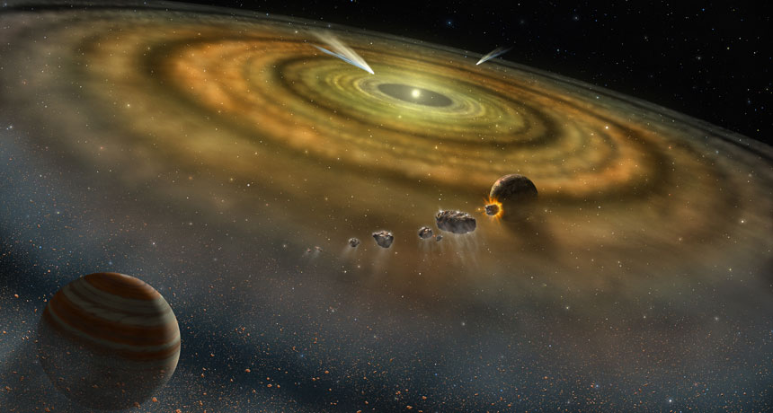
In other star systems, some moons could escape their planets and start orbiting their stars instead, new simulations suggest. Scientists have dubbed such liberated worlds “ploonets,” and say that current telescopes may be able to find the wayward objects.

Astronomers think that exomoons — moons orbiting planets that orbit stars other than the sun — should be common, but efforts to find them have turned up empty so far (SN Online: 4/30/19). Astrophysicist Mario Sucerquia of the University of Antioquia in Medellín, Colombia and colleagues simulated what would happen to those moons if they orbited hot Jupiters, gas giants that lie scorchingly close to their stars (SN: 7/8/17, p. 4). Many astronomers think that hot Jupiters weren’t born so close, but instead migrated toward their star from a more distant orbit.
As the gas giant migrates, the combined gravitational forces of the planet and the star would inject extra energy into the moon’s orbit, pushing the moon farther and farther from its planet until eventually it escapes, the researchers report June 27 at arXiv.org.

“This process should happen in every planetary system composed of a giant planet in a very close-in orbit,” Sucerquia says. “So ploonets should be very frequent.”

Some ploonets may be indistinguishable from ordinary planets. Others, whose orbits keep them close to their planet, could reveal their presence by changing the timing of when their neighbor planet crosses, or transits, in front of the star. The ploonet should stay close enough to the planet that its gravity can speed or slow the planet’s transit times. Those deviations should be detectable by combining data from planet-hunting telescopes like NASA’s TESS or the now-defunct Kepler, Sucerquia says.
Ploonethood may be a relatively short-lived phenomenon, though, making the worlds more difficult to spot. About half of the ploonets in the researchers’ simulations crashed into either their planet or star within about half a million years. And half of the remaining survivors crashed within a million years.

Even with few visible survivors, ploonets could help explain some bizarre exoplanetary features. Moon debris from such crashes could lead to giant ring systems around planets, like the 37 rings that encircle exoplanet J1407b, the team says.

Or, if the ploonet had an icy surface or an atmosphere before moving close to its star, the star’s heat would evaporate it, giving the ploonet a tail like a comet’s. Evaporating ploonets zipping by with a long light-blocking tail could explain strangely flickering stars like Tabby’s star, Sucerquia says (SN: 12/22/18, p. 9).

“Those structures [rings and flickers] have been discovered, have been observed,” Sucerquia says. “We just propose a natural mechanism to explain [them].”

While the solar system doesn’t have any hot Jupiters, ploonethood may be possible here, too. Earth’s moon is moving slowly away from the Earth, at a rate of about 4 centimeters per year. When it eventually breaks free, “the moon is a potential ploonet,” Sucerquia says — although that won’t happen for about 5 billion years.

The study is a good first step for thinking about what would happen to exomoons in real planetary systems, says planetary astrophysicist Natalie Hinkel of the Southwest Research Institute in San Antonio, who wasn’t involved in the new work. “Nobody’s looked at the problem quite like this,” she says. “It adds to the layers of how complex these systems are.”

Plus, ploonet is “a wonderful name,” Hinkel says. “Normally I sort of eye-roll at these made-up names, but this one is a keeper.”

Look up at the moon and you’ll see roughly the same patterns of light and shadow that Plato saw about 2,500 years ago. But humankind’s understanding of Earth’s nearest neighbor has changed considerably since then, and so have the ways that scientists and others have visualized the moon.

To celebrate the 50th anniversary of the Apollo 11 moon landing, here are a collection of images that give a sense of how the moon has been depicted over time — from hand-drawn illustrations and maps, to early photographs, to highly detailed satellite images made possible by spacecraft such as NASA’s Lunar Reconnaissance Orbiter.
The images, compiled with help from Marcy Bidney, curator of the American Geographical Society Library at the University of Wisconsin–Milwaukee, show how developments in technology such as the telescope and camera drove ever more detailed views of Earth’s closest celestial companion.

1. Atlas Coelestis, Johann Gabriel Doppelmayr, 1742
   Ancient Greek philosophers like Plato thought the moon and other celestial bodies revolved around a fixed Earth. This 1742 diagram by German scientist Johann Gabriel Doppelmayr depicts that idea. The thinkers saw the moon as perfect and struggled to explain its dark marks. In 1935, one of the moon’s most conspicuous craters was named after Plato.
2. Astronomicum Caesareum, Michael Ostendorfer, 1540
   This hand-colored woodcut by German painter Michael Ostendorfer appears in Astronomicum Caesareum, a vast collection of astronomical knowledge compiled by the German author Petrus Apianus and published in 1540. The image is an example of how astronomers in this early Renaissance period began to stylize the moon by giving it a face, Bidney says.

The book also contains more than 20 exquisitely detailed moving paper instruments, or volvelles, that helped predict lunar eclipses, calculate the position of the stars and more.

3. De Mundo, William Gilbert, ca. 1600
   Created around 1600, this sketch is the oldest known lunar map, and was drawn using the naked eye. William Gilbert, physician to Queen Elizabeth I, imagined that the bright spots were seas and the dark spots land, and gave some features names, such as Regio Magna Orientalis, which translates as “Large Eastern Region” and roughly coincides with the vast lava plain known today as Mare Imbrium.
4. Sidereus Nuncius, Galileo, 1610
   The telescope made it far easier to see the moon’s topography. By Galileo, these 1610 lunar maps are some of the first published to rely on telescope views. His work supported the Copernican idea that the moon, Earth and other planets revolved around the sun.

Although Galileo’s moon drawings were not the first to rely on telescope observations — English astronomer Thomas Harriot created the first sketch in 1609 — Galileo’s were the first published. These images appeared in his astronomical treatise Sidereus Nuncius.

5. Selenographia, Johannes Hevelius, 1647
   In 1647, Polish astronomer Johannes Hevelius, published the first lunar atlas, Selenographia. The book contains more than 40 detailed drawings and engravings, including this one, that show the moon in all its phases. Hevelius also included a glossary of 275 named surface features.

To create his images, Hevelius, a wealthy brewer, constructed a rooftop observatory in Gdańsk and fitted it with a homemade telescope that magnified the moon 40 times. Hevelius is credited with founding the field of selenography, the study of the moon’s surface and physical features.

6. First known lunar photo, John William Draper, 1840
   Photography opened a new way to capture the moon. Taken around 1840 by British-born chemist and physician John William Draper, this daguerreotype is the first known lunar photo. Spots are from mold and water damage.
7. “Moon over Hastings”, Henry Draper, 1863
   Photos of the moon quickly improved. John William Draper’s son Henry, a physician like his father, also developed a passion for photographing the night sky. He shot this detailed image from his Hastings-on-Hudson observatory in New York in 1863, and went on to become a pioneer in astrophotography.
8. Lunar Reconnaissance Orbiter, NASA, 2018
   This 2018 image, from NASA’s Lunar Reconnaissance Orbiter, shows the moon’s familiar face in incredible detail. Now we know its marks are evidence of a violent past and include mountain ranges, deep craters and giant basins filled with hardened lava.
9. Lunar farside, Chang’e-4, 2019
   Countless images now exist of the moon’s illuminated face, but only relatively recently have astronomers managed to capture shots of the moon’s farside, using satellites. Then in February, China’s Chang’e-4 lander and rover became the first spacecraft to land there. This is the first image captured by the probe.

By mounting a water distillation system on the back of a solar cell, engineers have constructed a device that doubles as an energy generator and water purifier.

While the solar cell harvests sunlight for electricity, heat from the solar panel drives evaporation in the water distiller below. That vapor wafts through a porous polystyrene membrane that filters out salt and other contaminants, allowing clean water to condense on the other side. “It doesn’t affect the electricity production by the [solar cell]. And at the same time, it gives you bonus freshwater,” says study coauthor Peng Wang, an engineer at King Abdullah University of Science and Technology in Thuwal, Saudi Arabia.
Solar farms that install these two-for-one machines could help meet the increasing global demand for freshwater while cranking out electricity, researchers report online July 9 in Nature Communications.

Using this kind of technology to tackle two big challenges at once “is a great idea,” says Jun Zhou, a materials scientist at Huazhong University of Science and Technology in Wuhan, China, not involved in the work.

In lab experiments under a lamp whose illumination mimics the sun, a prototype device converted about 11 percent of incoming light into electricity. That’s comparable to commercial solar cells, which usually transform some 10 to 20 percent of the sunlight they soak up into usable energy (SN: 8/5/17, p. 22). The researchers tested how well their prototype purified water by feeding saltwater and dirty water laced with heavy metals into the distiller. Based on those experiments, a device about a meter across is estimated to pump out about 1.7 kilograms of clean water per hour.

“It’s really good engineering work,” says George Ni, an engineer who worked on water distillation while a graduate student at MIT, but was not involved in the new study.
“The next step is, how are you going to deploy this?” Ni says. “Is it going to be on a roof? If so, how do you get a source of water to it? If it’s going to be [floating] in the ocean, how do you keep it steady” so that it isn’t toppled by waves? Such practical considerations would need to be hammered out for the device to enter real-world use.

A praying mantis depends on precision targeting when hunting insects. Now, scientists have identified nerve cells that help calculate the depth perception required for these predators’ surgical strikes.

In addition to providing clues about insect vision, the principles of these cells’ behavior, described June 28 in Nature Communications, may also lead to advances in robot vision or other automated systems.

So far, praying mantises are the only insects known to be able to see in 3-D. In the new study, neuroscientist Ronny Rosner of Newcastle University in England and colleagues used a tiny theater that played praying mantises’ favorite films — moving disks that mimic bugs. The disks appeared in three dimensions because the insects’ eyes were covered with different colored filters, creating minuscule 3-D glasses.
As a praying mantis watched the films, electrodes monitored the behavior of individual nerve cells in the optic lobe, a brain structure responsible for many aspects of vision. There, researchers found four types of nerve cells that seem to help merge the two different views from each eye into a complete 3-D picture, a skill that human vision cells use to sense depth, too.

One cell type called a TAOpro neuron possesses three elaborate, fan-shaped bundles that receive incoming visual information. Along with the three other cell types, TAOpro neurons are active when each eye’s view of an object is different, a mismatch that’s needed for depth perception.

The details of the various types of nerve cells, and how they might receive, combine and send visual information, suggest that these insects’ vision may be more sophisticated than some scientists had thought, the team writes. And the principles guiding praying mantis depth perception may be useful to researchers working on improving machine vision, perhaps allowing artificial systems to better sense the depths of objects.

Astronomy lovers are not the only ones excited about the 50th anniversary of the moon landing. Publishers are also taking note, serving up a pile of books to mark the occasion.

Are you looking for a general overview of the birth of the U.S. space program? Would you rather geek out on the technical details of the Apollo missions? How about flipping through a collection of photographs from the era? Science News staff took a look at the offerings and picked out a few favorites to help you decide. There’s something for everyone in the list below.
For history aficionados
James Donovan
Little, Brown and Co., $30

This retelling of the space race begins with the launch of the Soviet Union’s Sputnik satellite in 1957 and culminates in the historic Apollo 11 mission 12 years later. The book offers insights into the personalities of the astronauts, engineers and others who made the U.S. space program a success.
For detail-obsessed NASA fans
Charles Fishman
Simon & Schuster, $29.99

Getting to the moon demanded a million hours of work for each hour spent in space, this book argues. Accordingly, the story focuses on the engineers, coders, project managers and others who toiled to get the Apollo program off the ground.
For anyone who ever dreamed of being an astronaut
J.L. Pickering and John Bisney
Univ. of Florida, $45

Packed with hundreds of photos, some published for the first time, this coffee-table book reads like a photo album of the Apollo 11 mission. The images focus on candid moments from astronaut training, as well as the excitement of liftoff, the historic landing and the return home of the three men.

For readers ready for a sober view of Apollo
Roger D. Launius
Smithsonian Books, $27.95

A space historian takes the Apollo program off its pedestal to examine it from multiple angles: as a cog in the Cold War political machine, an engineering endeavor riddled with as many failures as feats of glory and an iconic cultural moment. The book explores both positive and negative viewpoints on the U.S. moonshot project from scientists, politicians, the media and the public during the space race and beyond.

For fans of graphic novels
Jonathan Fetter-Vorm
Hill and Wang, $35

Colorful and detailed, the comic-style illustrations in this book of graphic nonfiction bring the moon landing to life. Much of the astronauts’ dialog is based on real recordings, making the book feel particularly authentic.

For self-improvement buffs
Richard Wiseman
TarcherPerigee, $26

A psychologist takes practical lessons from the Apollo era and suggests ways to apply them to everyday problems, from changing careers to raising a family.

For space enthusiasts
David Baker
Arcturus Publishing Limited, $19.99

A former NASA engineer uses photographs, illustrations, blueprints and other documents to guide readers through a concise history of the space race and the Apollo program, from the beginnings of rocket science to the successful return home of the Apollo 11 crew.

For history wonks with a soft spot for psychology
Basil Hero
Grand Central Publishing, $22

The Apollo astronauts rarely gave personal interviews. But now that they’re getting older, the astronauts are starting to get introspective. This book distills conversations with the 12 lunar voyagers still alive into general wisdom on conquering fear and appreciating life.

For photography lovers
Deborah Ireland
Ammonite Press, $14.95

This slim book offers an offbeat take on the mission to the moon, telling the story of the Apollo program through the development of the Hasselblad cameras that Neil Armstrong and Buzz Aldrin used to document their time on the lunar surface.
Science News is a participant in the Amazon Services LLC Associates Program. Please see our FAQ for more details.