SAN DIEGO — A nerve-zapping headset caused people to shed fat in a small preliminary study.
Six people who had received the stimulation lost on average about 8 percent of the fat on their trunks in four months, scientists reported November 12 at the annual meeting of the Society for Neuroscience.
The headset stimulated the vestibular nerve, which runs just behind the ears. That nerve sends signals to the hypothalamus, a brain structure thought to control the body’s fat storage. By stimulating the nerve with an electrical current, the technique shifts the body away from storing fat toward burning it, scientists propose. Six overweight and obese people received the treatment, consisting of up to four one-hour-long sessions of stimulation a week. Because it activates the vestibular system, the stimulation evoked the sensation of gently rocking on a boat or floating in a pool, said study coauthor Jason McKeown of the University of California, San Diego.
After four months, body scans measured the trunk body fat for the six people receiving the treatment and three people who received sham stimulation. All six in the treatment group lost some trunk fat, despite not having changed their activity or diet. In contrast, those in the sham group gained some fat. Researchers suspect that metabolic changes are behind the difference. “The results were a lot better than we thought they’d be,” McKeown said.
Earlier studies had found that vestibular nerve stimulation causes mice to drop fat and pack on muscle, resulting in what McKeown called Schwarzenegger mice. Though small, the current study suggests that the approach has promise in people. McKeown and colleagues have started a company based on the technology and plan to test it further, he said.
SAN ANTONIO — Early Christian monks’ vows of silence may have attracted not only the devout but also a fair number of hearing-impaired men with a sacred calling.
A team led by bioarchaeologist Margaret Judd of the University of Pittsburgh found that a substantial minority of Byzantine-era monks buried in a communal crypt at Jordan’s Mount Nebo monastery display skeletal signs of hearing impairments. Judd presented these results November 19 at the annual meeting of the American Schools of Oriental Research. Judd has directed excavations at Mount Nebo since 2007. Her new results focus on a two-chambered crypt containing skeletons of at least 57 men presumed to have been monks. Oil lamps found in the crypt date to the 700s.
About 16 percent of these men displayed damage to middle ear bones caused by infections known as otitis media. This condition frequently occurs in childhood and can lead to lasting hearing problems even if the infection clears up quickly (SN Online: 3/10/10). Monks showing signs of otitis media probably suffered mild to moderate hearing loss.
Damage to one middle ear bone, the stapes, in two other individuals likely caused severe hearing loss in one ear each. In another case, a fracture above the left eye could have damaged middle ear bones, Judd proposed. Finally, one skull’s thickened bone may have resulted from Paget’s disease, a viral infection in adulthood that can impair hearing.
Hearing loss would have had little effect on monks’ daily lives, since they communicated with hand signals, nods and other gestures, Judd said. Even if some developed hearing ailments after joining the monastery, those conditions must have largely gone undetected by affected monks and their peers who rarely or never spoke, she suggested.
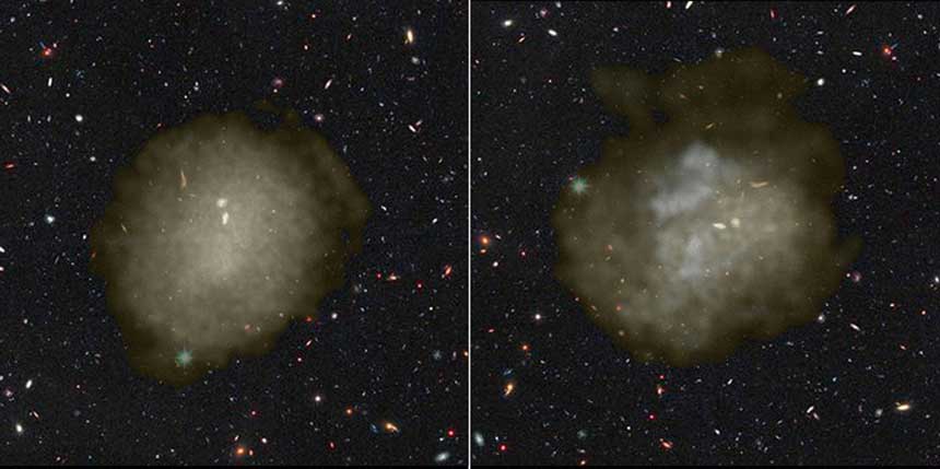
Brilliant births and destructive deaths of stars might take a runt of a galaxy and stretch it to become a ghostly behemoth, new computer simulations show. This process could explain the origin of recently discovered dark galaxies, which can be as wide as the Milky Way but host roughly 1 percent as many stars.
Since 2015, astronomers have found hundreds of these shadowy systems lurking in and around several clusters of galaxies (SN: 12/10/16, p. 18). How these dark galaxies form is a puzzle. But prolific star formation and blast waves from exploding stars could be responsible, researchers suggest in a paper to appear in Monthly Notices of the Royal Astronomical Society Letters. “The mystery is: Are these galaxies like the Milky Way, or are they dwarf galaxies?” says study coauthor Arianna Di Cintio, an astrophysicist at the University of Copenhagen in Denmark. “Our mechanism could be a nice formation scenario for these galaxies and prove that they are dwarfs.”
Di Cintio and colleagues ran computer simulations of galaxy evolution and found that some runts can be inflated by stellar energy. Radiation from young massive stars heats up interstellar gas, preventing it from forming more stars. And a flurry of supernova explosions can toss that gas out of the galaxy. The gravity of the galaxy drops, and so does its ability to hold on to stars and dark matter, an enigmatic substance thought to help hold galaxies together. “Dark matter particles fly outward and start the expansion,” says Di Cintio. “This happens to the stellar population as well.”
Those galaxies that remain as runts in the simulations go through this process just once, whereas giant dark galaxies regurgitate their gas multiple times. And that provides a way to test this idea, says Di Cintio. First astronomers need to find dark entities far away from galaxy clusters where the environment can also take its toll. Then researchers can estimate the ages of stars in the galaxy to see if there have been multiple bursts of star formation. If this hypothesis is correct, dark galaxies might also be loaded up with lots of hydrogen gas that allows them to sustain several rounds of gas purging.
“It is very interesting to see that, in some cases, [supernovas] can be efficient enough to expand dwarf galaxies,” says Nicola Amorisco, also at the University of Copenhagen. He helped put forth an idea that dark galaxies start as runts that get stretched because of rapid rotation. Recent observations also show that some dark systems have masses that are similar to dwarf galaxies (though one is as hefty as the Milky Way). “It is even possible that a combination of — or the interplay between — a few different mechanisms could be responsible,” says Amorisco. “It will be very exciting to understand whether that is the case.”
At first glance, the stories taking the top two spots in Science News’ review of 2016 have little in common. Scientists began searching decades ago for gravitational waves. Discussions of these subtle signals from dramatic and distant phenomena appear dozens of times in the SN archive starting as early as the 1950s. Their long-awaited discovery, our No. 1 story of the year, touched off celebration of a new era in astronomy.
Less expected, and far from subtle, was the sudden rise in Brazil of microcephaly cases, linked this year to Zika virus infections — our No. 2 story. Little was known about Zika before the outbreak, which delivered devastation and fear across the Americas. In fact, only a single previous mention of Zika exists in the SN archive, in a book review from the 1990s. But the stories have at least one thing in common: Both highlight the power of scientific discoveries to trigger our deepest human emotions. Pure elation as well as overwhelming dread can accompany research advances.
2016 brought many more sentiments, too. There was enthusiasm for the discovery of the exoplanet Proxima b, concern for the prospects of three-parent babies and feelings of potential but also impending peril in the openings of Arctic passageways.
The editors and writers at Science News also recognize that some of the best and most moving stories are those that are still unfolding. So, in addition to the discoveries of 2016, we review milestones, setbacks and other tales of unsteady progress. Sonia Shah writes about a new wave of infectious diseases; Tom Siegfried explores convergent failures in the field of particle physics; and Laurel Hamers covers key challenges for self-driving cars. Then, Science News writers share what science news they’re most excited about in the year to come. — Elizabeth Quill
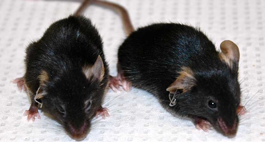
Four proteins that can transform adult cells into embryonic-like ones can also turn back the aging clock, a new study in mice suggests.
Partial reprogramming of cells within prematurely aging mice’s bodies extended the rodents’ average life span from 18 weeks to 24 weeks, researchers report December 15 in Cell. Normal mice saw benefits, too: Muscles and pancreas cells healed better in middle-aged mice that got rejuvenation treatments than in mice that did not. The experiment could be evidence that epigenetic marks — chemical tags on DNA and proteins that change with age, experience, disease and environmental exposures — are a driving factor of aging. Some marks accumulate with age while others are lost. “It’s an inspiring paper,” says Jan van Deursen, a biologist at the Mayo Clinic in Rochester, Minn., who studies diseases of aging. He gives the paper an “A” for sparking imagination, but lower marks for practical applications to human aging because it would involve gene therapy and could be risky. “It’s all cool, but I don’t see that it could ever be applied in medicine,” he says. “We could be terribly wrong. Hopefully we are.”
Researchers reset the mice’s aging clock by genetically engineering the animals to make four proteins when the rodents were treated with the antibiotic doxycycline. Those four proteins — Oct4, Sox2, Klf4 and c-Myc — are known as “Yamanaka factors” after Shinya Yamanaka. The Nobel Prize‒winning scientist demonstrated in 2006 that the proteins could turn an adult cell into an embryonic-like cell known as an induced pluripotent stem cell, or iPS cell (SN: 11/3/12, p. 13; SN: 7/14/07, p. 29). The factors help strip away epigenetic marks that enable cells to know whether they are heart, brain, muscle or kidney cells, for example. As a result, stripped cells revert to the ultraflexible pluripotent state and are capable of becoming nearly any type of cell. Other researchers have used the Yamanaka factors to reprogram cells within living mice before, but those attempts resulted in the growth of tumors. (Cancer cells resemble stem cells in that they don’t have a specific identity and are “undifferentiated.”) Those tumors indicated to Alejandro Ocampo and colleagues that the proteins were rewriting epigenetic programming to take cells back to an undifferentiated state. But “you don’t need to go all the way back to pluripotency” to erase the marks associated with aging, says Ocampo, a stem cell biologist at the Salk Institute for Biological Studies in La Jolla, Calif. A milder reprogramming treatment might reverse aging without stripping away cells’ identity, leading to cancer, Ocampo and colleagues thought.
The researchers put genetically engineered mice with a premature aging disease called progeria on a regimen in which the animals were treated with doxycycline two days per week to turn on the Yamanaka factors. Mice that made the reprogramming proteins lived six weeks longer on average than mice that didn’t get the treatment. The mice didn’t get cancer, but still died prematurely (lab mice usually live two to three years on average). “We are far away from perfection,” Ocampo says.
Normally aging mice also got benefits from the treatment. When the animals were 1 year old (roughly middle-aged), the researchers treated them with doxycycline two days per week for three weeks. Treated mice were better able to repair muscles and replace insulin-producing cells in the pancreas than untreated mice. Not all organs fared as well, Ocampo says, citing preliminary evidence. Ongoing experiments will determine whether the epigenetic reprogramming can make the mice live any longer or healthier. People probably won’t be genetically engineered the way mice are. But chemicals and small molecules might also be able to wipe away epigenetic residue that builds up with aging and restore marks that were lost over time, returning to a pattern seen in youth, Ocampo suggests.
Researchers still don’t know whether all cells are rejuvenated by the treatment. Yamanaka factors may breathe new life into aging stem cells, allowing them to replenish damaged tissues. Or the factors may wake up senescent cells — cells that have shut down normal functions and cease to divide, but may send signals to neighboring cells that cause them to age (SN: 3/5/16, p. 8). Reviving senescent cells could be dangerous, says van Deursen; the body shuts cells down to prevent them from becoming cancerous.
Plenty of evidence indicates that resetting epigenetic programming can extend life, says Ocampo. He points to a recent report that Dolly the Sheep’s cloned sisters are aging normally (SN: 8/20/16, p. 6) as a hopeful sign that reprogramming probably isn’t dangerous, and might one day safely prevent many of the diseases associated with aging in people, if not lengthening life spans.
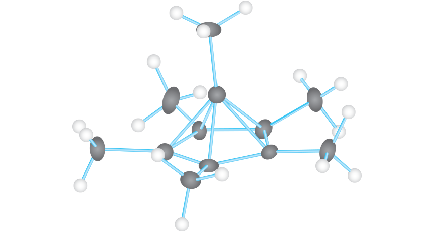
A molecule originally proposed more than 40 years ago breaks the rules about how carbon connects to other atoms, scientists have confirmed. In this unusual instance, a carbon atom bonds to six other carbon atoms. That structure, mapped for the first time using X-rays, is an exception to carbon’s textbook four-friend limit, researchers report in the Jan. 2 Angewandte Chemie.
Although the idea for the structure isn’t new, “I think it has a larger impact when someone can see a picture of the molecule,” says Dean Tantillo, a chemist at the University of California, Davis who wasn’t part of the study. “It’s super important that people realize that although we’re taught carbon can only have four friends, carbon can be associated with more than four atoms.” Atoms bond by sharing electrons. In a typical bond two electrons are shared, one from each of the atoms involved. Carbon has four such sharable electrons of its own, so it tends to form four bonds to other atoms.
But that rule doesn’t always hold. In the 1970s, scientists made an unusual discovery about a molecule called hexamethylbenzene. This molecule has a flat hexagonal ring made of six carbon atoms. An extra carbon atom sticks off each vertex of the ring, like six tiny arms. Hydrogen atoms attach to the ring’s arms. And leftover electrons zip around the middle of the ring, strengthening the bonds and making the molecule more stable. When the scientists removed two electrons from the molecule, leaving it with a positive charge, some evidence suggested it might dramatically change its shape. It seemed to rearrange so that one carbon atom was bonded to six other carbons. But the researchers didn’t experimentally confirm that structure. Now, a different lab has revisited the question. Making this charged version of hexamethylbenzene is a challenge because it’s stable only in extremely strong acid, says study coauthor Moritz Malischewski, a chemist at the Free University of Berlin. And the experimental details in the old study were a bit fuzzy. But after a bit of tinkering, he managed to create the charged molecule. He and coauthor Konrad Seppelt crystallized it with some other molecules, and then used X-rays to get a three-dimensional map of the crystal structure.
The X-ray experiment confirmed what other scientists had suggested in the 1970s: When hexamethylbenzene lost two electrons, it reordered itself. One carbon atom jumped out of the ring and took a new position on top, turning the flat hexagonal ring into a five-sided carbon pyramid. And the carbon on top of the pyramid was indeed bonded to six other carbons — five in the ring below, and one above.
“This molecule is very exceptional,” says Malischewski. Though scientists have found other exceptions to carbon’s four-bond limit, this is the first time carbon has been shown associating with this many other carbon atoms.
When Malischewski measured the length of the molecule’s chemical bonds, the top carbon’s six bonds were each a bit longer than an ordinary carbon-carbon bond. A longer bond is generally less strong. So by picking more partners, that carbon has a slightly weaker connection to each one.
“The carbon isn’t making six bonds in the sense that we usually think of a carbon-carbon bond as a two-electron bond,” Tantillo says. That’s because the carbon atom still has only four electrons to share. As a result, it spreads itself a bit thin by sharing electrons among the six bonds.
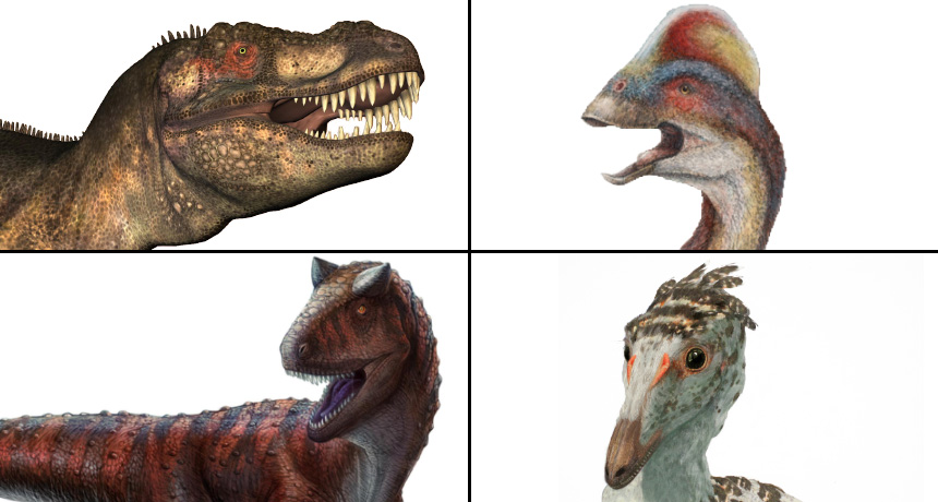
Dinosaur fashion, like that of humans, is subject to interpretation. Bony cranial crests, horns or bumps may have served to woo mates or help members of the same species identify one another. While the exact purpose of this skull decor is debated, the standout structures tended to come with an even more conspicuous trait: bigger bodies.
Terry Gates, a paleontologist at North Carolina State University in Raleigh, and colleagues noticed an interesting trend in the fossil record of theropods, a group of dinosaurs that includes Tyrannosaurus rex and the ancestors of birds. Bigger beasts often sported skeletal headgear. Across the family tree, Gates and his team analyzed 111 fossils dating from 65 million to 210 million years ago, and the trend held true. It makes sense: “Dinosaur size matters in terms of how they will be visually talking to one another,” says Gates. “When you’re smaller, your means of visual communication would be different than when you’re giant.”
The researchers also calculated that over time, theropod lineages with head ornaments evolved giant bodies (larger than 1,000 kilograms) 20 times faster on average than those without. Ornaments might have supersized some dinos, but researchers aren’t sure. The analysis, which appeared September 27 in Nature Communications, suggests theropods had to reach at least 55 kilograms to grow the headgear.
But among big-boned relatives of modern birds, skull toppers weren’t in vogue. Many of these dinos grew heavier than 55 kilograms, but they instead sported feathers that resembled those used by modern birds for flight. That might be because bigger, bolder feathers and showy headwear served similar ends. Gates speculates: “Once you have a signaling device in the form of a feather, why grow a bony cranial crest?” For these plumed dinosaurs, feathers were in and bony ornaments were out.
Size matters Many large theropods, a group of dinosaurs that includes Tyrannosaurus rex and the ancestors of birds, had bony head ornaments such as crests, horns and bumps. New research suggests theropods had to reach at least 55.2 kilograms to grow the cranial decor. But big-boned dinos related to modern birds lacked the ornaments. Instead, they were decked out in feathers resembling those used by modern birds for flight.
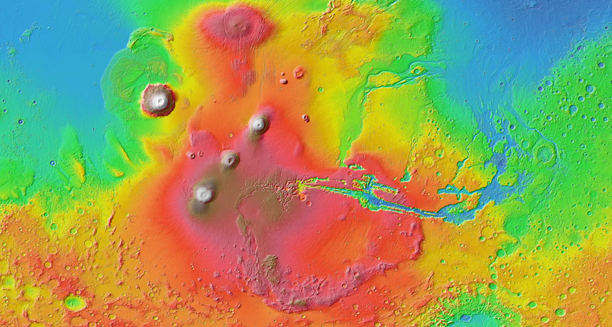
An enduring source of magma on Mars fueled volcanic eruptions for billions of years, clues inside a rock flung from the Red Planet reveal.
The newfound rock belongs to a batch of meteorites called shergottites that originated from the same Martian volcanic system, researchers report February 1 in Science Advances. But the new rock is considerably older than its counterparts. While previously discovered shergottites solidified from Martian magma between 427 million and 574 million years ago, the new rock formed around 2.4 billion years ago, chemical analyses show. Such a wide range of ages means that a volcanic system on Mars churned out hot rocks from a stable source of magma for nearly half of the planet’s history, says study coauthor Thomas Lapen, a geologist at the University of Houston. That endurance could help scientists better understand Mars’ interior. “These are some of the longest-lived volcanoes in the solar system,” Lapen says.
Lapen and colleagues studied elements inside a Martian meteorite discovered in Algerian desert in 2012. Some of those elements serve as stopwatches that record the history of the rock. Isotopes of beryllium and aluminum, formed during exposure to cosmic rays, reveal that the rock zipped through space for around 1 million years. The steady decay of carbon 14 — left behind after cosmic ray collisions — suggests that the rock landed on Earth roughly 2,300 years ago. By combining these two measurements, the researchers found that the meteorite probably blasted off Mars alongside other shergottites a little over a million years ago. This exodus probably followed a massive impact in Mars’ volcano-filled Tharsis region. The rocks share more than their exit route, the researchers found. Chemical similarities between the meteorites suggest that they all originate from the same source of hot rock deep within the Red Planet. That’s surprising given that the mix of radioactive elements inside the newfound meteorite suggests it solidified 1.8 billion years earlier than the next oldest shergottite, Lapen says.
Mars is known to have many volcanic systems across its surface, all fed by magma upwelling from the planet’s depths. Studies have previously suggested that some of these systems operated for billions of years. Though little is known about the Martian interior, many scientists had assumed that the magma feeding this volcanism changed over time as the Martian interior mixed. The absence of any difference in composition of the shergottites suggests Mars’ interior is relatively stagnant. That may result from Mars’ lack of plate tectonics, a process that helps blend Earth’s innards, Lapen proposes. Understanding the differences between Earth and Mars could help reveal why the two planets took such different trajectories, with Earth so much more life-friendly than Mars (SN: 5/2/15, p. 24). Similarities between the shergottites could have another explanation, says planetary scientist Stephanie Werner of the University of Oslo. Large impacts can melt rocks, resetting their age. The shergottites may have formed around the same time billions of years ago before some had their ages altered by impacts over time, she proposes.
Upcoming missions will help illuminate what’s going on beneath the Martian surface, says James Head, a planetary scientist at Brown University in Providence, R.I. NASA’s InSight lander, currently slated for launch in 2018, will use seismic activity to map the Red Planet’s interior.
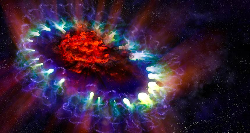
In A.D. 185, Chinese records note the appearance of a “guest star” that then faded away over the span of several months. In 1572, astronomer Tycho Brahe and many others watched as a previously unknown star in the constellation Cassiopeia blasted out gobs of light and then eventually disappeared. And 30 years ago, the world witnessed a similar blaze of light from a small galaxy that orbits the Milky Way. In each case, humankind stood witness to a supernova — an exploding star — within or relatively close to our galaxy (representative border in gray, below).
Here’s a map of six supernovas directly seen by human eyes throughout history, and one nearby explosion that went unnoticed. Some were type 1a supernovas, the detonation of a stellar core left behind after a star releases its gas into space. Others were triggered when a star at least eight times as massive as the sun blows itself apart.
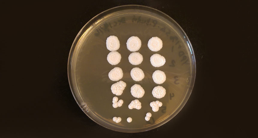
BOSTON — A fungus among us may tip the body toward developing asthma.
There’s mounting evidence that early exposure to microbes can protect against allergies and asthma (SN Online: 7/20/16). But “lo and behold, some fungi seem to put kids at risk for asthma,” microbiologist Brett Finlay said February 17 at a news conference during the annual meeting of the American Association for the Advancement of Science.
Infants whose guts harbored a particular kind of fungus — a yeast called Pichia — were more likely to develop asthma than babies whose guts didn’t have the fungus, Finlay reported. Studies in mice and people suggest that exposure to some fungi can both trigger and exacerbate asthma, but this is the first work linking asthma to a fungus in the gut microbiome of infants. Finlay, of the University of British Columbia in Vancouver, and his colleagues had recently identified four gut bacteria in Canadian infants that seem to provide asthma protection. To see if infants elsewhere were similarly protected by such gut microbes, he decided to look at another population of children with an asthma rate similar to Canada’s (about 10 percent). He and his colleagues sampled the gut microbes of 100 infants in rural Ecuador and followed up five years later.
The researchers identified several factors that might influence risk of developing asthma, such as exposure to antibiotics, having respiratory infections, and whether or not the infants were breastfed. Of the 29 infants in the high-risk asthma group, more than 50 percent had asthma by age 5, Finlay said.
Surprisingly, the strongest predictor of whether a child developed asthma wasn’t bacterial. It was the presence of Pichia. And the yeast wasn’t protective; it tipped the scales toward asthma.
Finlay speculated that molecules made by the fungi interact with the infants’ developing immune systems in a way that somehow increases asthma risk. It isn’t clear how the infants’ guts acquire the fungus; some species of Pichia are found in soil, others in raw milk and cheese. Finlay and his colleagues are now going to look for the fungus in Canadian children’s gut microbes..
The researchers also looked at other gut microbe‒related factors that upped the Ecuadorean children’s asthma risk. Children with access to clean water had higher asthma rates, Finlay said. While drinking clean water helps people avoid several ills such as cholera, the link to asthma highlights how some dirt can be protective, he said. “We’ve cleaned up our world too much.” This research underscores that caution should be used when generalizing about our intestinal flora. “What’s emerging is that it is very personalized,” gastroenterologist Eran Elinav of the Weizmann Institute of Science in Rehovot, Israel, said at the news conference. For example, evidence implicates some fungi in the development of inflammatory bowel disease, Elinav said, but it depends on the individual.